使用 Mini Batch K-Means 进行图像压缩

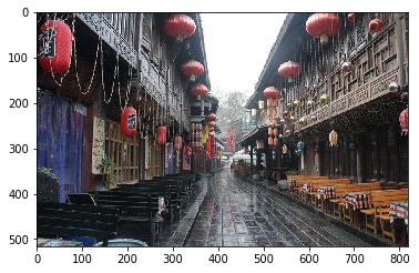
针对一张成都著名景点：锦里的图片，通过 Mini Batch K-Means 的方法将相近的像素点聚合后用同一像素点代替，以达到图像压缩的效果。

图像导入

\# 使用 Matplotlib 可视化示例图片  
%matplotlib inline  
import matplotlib.pyplot as plt   
import matplotlib.image as mpimg   
  
chengdu = mpimg.imread('chengdu.png') # 将图片加载为 ndarray 数组  
plt.imshow(chengdu) # 将数组还原成图像  

|

|

1  

|

chengdu.shape  

|

(516, 819, 3) 

在使用 mpimg.imread 函数读取图片后，实际上返回的是一个 numpy.array 类型的数组，该数组表示的是一个像素点的矩阵，包含长，宽，高三个要素。如成都锦里这张图片，总共包含了 516$516$ 行，819$819$ 列共 516⋅819=422604$516⋅819=422604$ 个像素点，每一个像素点的高度对应着计算机颜色中的三原色 R,G,B$R,G,B$（红，绿，蓝），共 3 个要素构成。

数据预处理

为方便后期的数据处理，需要对数据进行降维。

|

1  
2  
3  

|

\# 将形状为 (516, 819, 3) 的数据转换为 (422604, 3) 形状的数据。  
data = chengdu.reshape(516\*819, 3)  
data.shape, data\[10\]  

|

((422604, 3), array([0.12941177, 0.13333334, 0.14901961], dtype=float32)) 

像素点种类个数计算

尽管有 422604 个像素点，但其中仍然有许多相同的像素点。在此我们定义：R,G,B$R,G,B$ 值相同的点为一个种类，其中任意值不同的点为不同种类。

|

1  
2  
3  
4  
5  
6  
7  
8  
9  
10  
11  
12  
13  
14  
15  
16  
17  

|

"""计算像素点种类个数  
"""  
def get\_variety(data):  
    """  
    参数:  
    预处理后像素点集合  
  
    返回:  
    num\_variety -- 像素点种类个数  
      
    思路：将数据转化为 list 类型，然后将每一个元素转换为 tuple 类型，最后利用 set() 和 len() 函数进行计算。  
    """  
  
    temp = data.tolist()  
    num\_variety=len(set(\[tuple(t) for t in temp\]))  
      
    return num\_variety  

|
|

1  

|

get\_variety(data), data\[20\]  

|

(100109, array([0.24705882, 0.23529412, 0.2627451 ], dtype=float32)) 

Mini Batch K-Means 聚类

像素点种类的数量是决定图片大小的主要因素之一，在此使用 Mini Batch K-Means 的方式将图片的像素点进行聚类，将相似的像素点用同一像素点值来代替，从而降低像素点种类的数量，以达到压缩图片的效果。

|

1  
2  
3  
4  
5  
6  
7  
8  

|

from sklearn.cluster import MiniBatchKMeans  
  
model = MiniBatchKMeans(10) # 聚类簇数量设置为 10 类  
  
model.fit(data)  
predict=model.predict(data)  
  
new\_colors = model.cluster\_centers\_\[predict\]  

|
|

1  
2  

|

\# 调用前面实现计算像素点种类的函数，计算像素点更新后种类的个数  
get\_variety(new\_colors)  

|

10 

图像压缩前后展示

|

1  
2  
3  
4  
5  
6  

|

\# 将聚类后并替换为类别中心点值的像素点，变换为数据处理前的格式，并绘制出图片进行对比展示  
fig, ax = plt.subplots(1, 2, figsize=(16, 6))  
  
new\_chengdu = new\_colors.reshape(chengdu.shape)  
ax\[0\].imshow(chengdu)  
ax\[1\].imshow(new\_chengdu)  

|

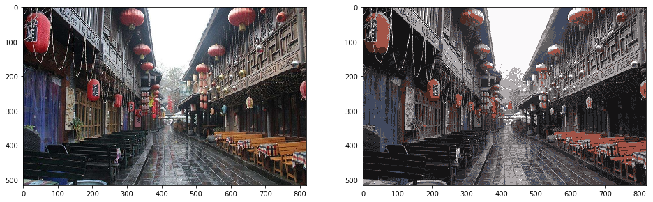
通过图片对比，可以十分容易发现画质被压缩了。其实，因为使用了聚类，压缩后的图片颜色就变为了 10 种。

接下来，使用 mpimg.imsave() 函数将压缩好的文件进行存储，并对比压缩前后图像的体积变化。

|

1  
2  
3  
4  

|

\# 运行对比  
mpimg.imsave("new\_chengdu.png",new\_chengdu)  
!du -h new\_chengdu.png  
!du -h chengdu.png  

|

220K    new_chengdu.png
1.1M    chengdu.png 

可以看到，使用 Mini Batch K-Means 聚类方法对图像压缩之后，体积明显缩小。